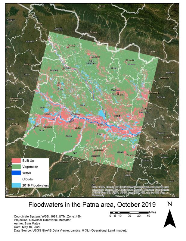
 In this project, I wanted to ascertain the extent of floodwaters near the city of Patna, in the Indian state of Bihar, in October 2019. (For more on this flood, see www.forbes.com/sites/lauratenenbaum/2019/10/15/climate-change-impacts-monsoon-flooding-in-india/). I used the USGS GloVis viewer to download two Landsat 8 raster images for an identical area including the city of Patna, from October 2015 (a time where there was no major flooding in the area) and October 2019. Notably, I made sure that these rasters were identical in their area coverage. I endeavored to find a closer chronological match for the pre-flooding raster, perhaps October 2018, but was limited by the need to find rasters that had reasonably low cloud cover. My question was “Which parts of the water-covered areas seen in the October 2019 raster are the result of floodwaters, as opposed to being normal for that time of year?” To answer this, I ran a supervised (trained) classification on the October 2019 raster, with four classes: Built Up (including everything from the urban center of Patna to villages), Vegetation (forests and agricultural land), Clouds, and Water. I then ran a Maximum Likelihood Classification, resulting in a classified raster. After noting some discrepancies, I changed several of my training samples and ran a new, more successful, Maximum Likelihood Classification. I then ran a Raster to Polygon tool, set to create multi-part polygons, and used Select by Attributes to extract the Water class as its own file. I then repeated this sequence of Maximum Likelihood Classification, Raster to Polygon, and Select by Attributes (extracting the water polygon) for the October 2015 raster. Notably, I used the same signature file I had created to train the classification of the October 2019 raster on the October 2015 raster, to ensure that the same pixel reflectance values were assigned to the same categories in both classifications. At this point, I had two polygons: one showing all water in the area from October 2019 and one showing all water in the area from October 2015. I used the Erase tool, with the 2019 water as the input feature and the 2015 water as the Erase feature, to return a polygon depicting all water that was present in the area in October 2019 but not in October 2015. (In total, seven geoprocessing steps were run in this analysis: two Maximum Likelihood Classifications, two Raster to Polygons, two Select by Attributes, and an Erase). These were, to a rough approximation, the floodwaters. I found that this covered a substantial area, visually indicating the abnormalities caused by the October 2019 flooding. I then created a model of this analysis process, with Pre-Flood Raster, Post-Flood Raster, Signature File, and Selection Expression as inputs. For any two rasters depicting the same area before and after a flood, this pattern can create a simple visualization of the extent of the floodwaters. Notably, the Selection Expression should be written down beforehand. My expression happened to be “gridcode=65,” based on the water samples in the signature file, but this will vary from analysis to analysis. I was quite pleased with the results. By overlaying the “Floodwaters” raster on the October 2019 classified raster, the extent of the flooding is very clearly visible. Adding a basemap allows direct comparison of flooded areas to on-the-ground localities, potentially making this analysis very useful for resource and aid distribution in the immediate aftermath of widespread floods. Particularly in parts of the world with poor communications or infrastructure, this kind of analysis could unveil underserved areas. One potential limitation is cloud cover-I selected two rasters with low cloud cover, but clouds covering varying parts of the area did add some uncertainty into the analysis. A potential follow-up analysis would be to find census data for the areas covered by floodwater, and calculate how many people were displaced by the floods.
0 Comments
Leave a Reply. |
|||
 RSS Feed
